Malware Detecting using Control Flow Graphs

By Edwin Huang, Sabrina Ho

Link to Webpage

Introduction

There are many malware detection tools available in the market, including pattern-based, behavior-based methods, etc, with the prompt development of artificial intelligence, many modern data analysis methods are applied to detecting malware in recent years. We are interested in investigating the effectiveness of different data analysis methods for detecting certain types of malware.

As the number of malicious software (malware) increases throughout the past few decades, malware detection has become a challenge for app developers, companies hosting the apps, and people using the apps. There are many pieces of research conducted on malware detection since it first appeared in the early 1970s. Just like the paper we studied in our first quarter, it uses the HIN (Heterogeneous Information Network) structure to classify the Android applications. It also compared its own method against other popular methods such as Naive Bayes and Decision Tree, and other known commercial mobile security products, to test its performance. The result showed that their method performs better than the other methods with an accuracy of 98% while other others only achieve an average of 90\%. After studying the paper, we are more curious about the detecting effectiveness of an analysis method when applied to a certain type of malware.

Not everyone has access to tools that can detect whether or not the app they just downloaded is malicious or not. Our motivation to conduct this research is to hope to produce a recommending tool that can be easily accessed by the general public for detecting malware. Optimistically, we want to reduce the chance of people downloading malicious apps and potentially prevent their devices from being hacked. To achieve that, we will be classifying applications using Control Flow Graphs and different similarity-based methods including k-nearest neighbors (kNN) as well as Random Forest classifier to see if different methods can detect certain types of malware or any specific features.

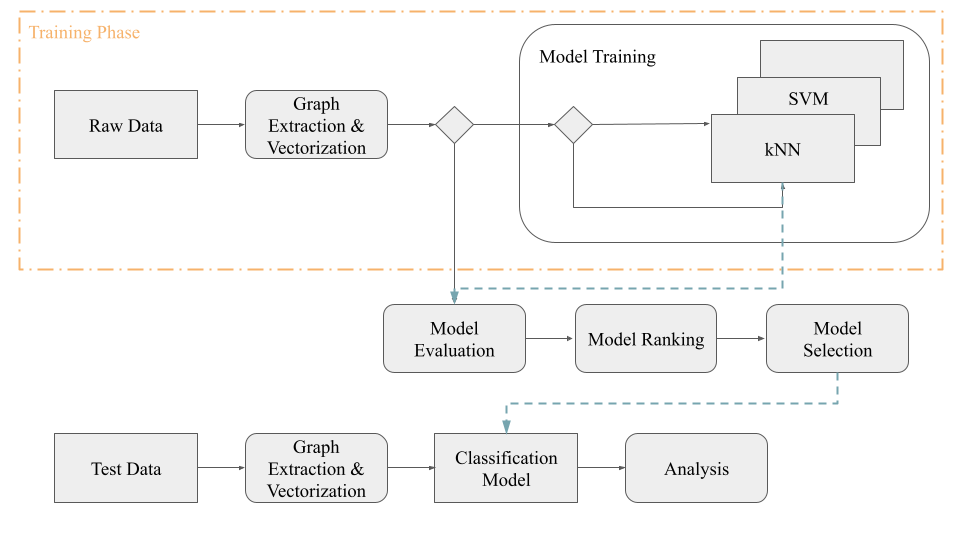
We are interested in analyzing whether one classifier has better performance in detecting certain types of malware or specific features, and designing a framework for recommending a method with a specific set of parameters for a certain type of malware and provide users a more friendly interface. With the similarity-based approach, we believe that it will detect malware with much higher accuracy and will be more flexible for applications that evolved over time as they become more complicated.

Related Work

Mamadroid

MamaDroid is a system that detects Android malware by the apps’ behaviors. This method extract call graphs from APKs, which are represented using nodes and edges in a graph object. From each graph, sequences of probabilities are extracted, representing one feature vector per APK. These probabilistic feature vectors are used for malware classification. MamaDroid also abstracts each API call to the family and package level, which inspired us to abstract to the class level. This is discussed further later.

Hindroid

Hindroid is a system that parses SMALI code extracted from APKs and uses them to create four different graphs, which are represented by large matrices. Within these matrices, each value in a matrix corresponds to an edge. A combination of these matrices are used to classify malicious software and benign apps.

Metapath2Vec

Metapath2Vec is a node representation learning model that uses predefined paths based on the node types. These paths define where the the program can traverse the graph. Following is an example of a metapath. In this case below, the metapath is Type 1 → Type 2 → Type 1 → Type 3 → Type 1.

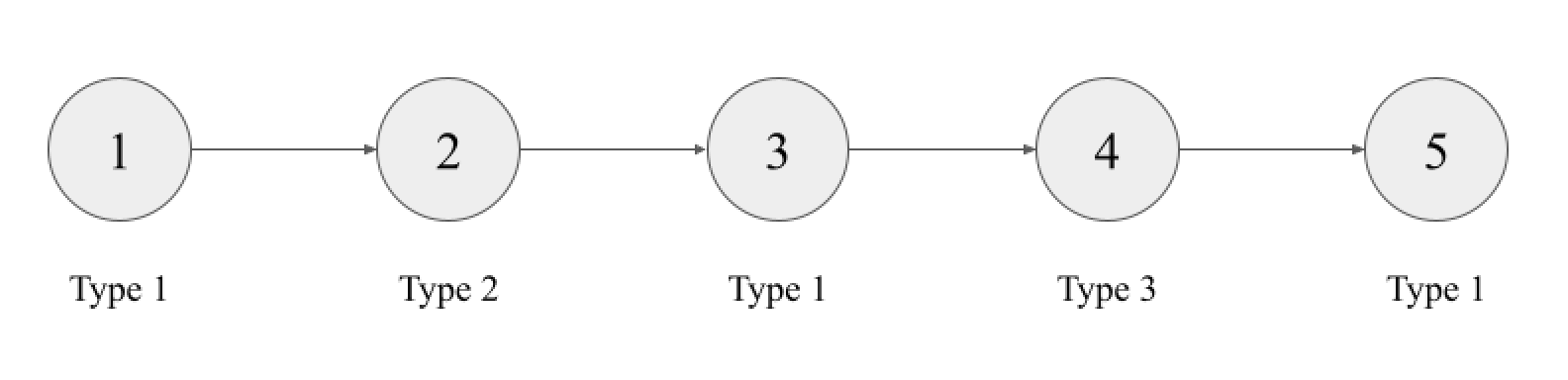
With predefined meta-paths, we can traverse a graph according to these node types to generate a large corpus, which is then fed into Node2Vec to obtain representations of words. This method will obtain one vector for one node within the graph.

Word2Vec

Word2vec is a model that turns text into numerical representations. It is trained on a large corpus, and outputs a representation for each word in the corpus. Below is a famous example of Word2Vec: King and Queen and Men and Women.

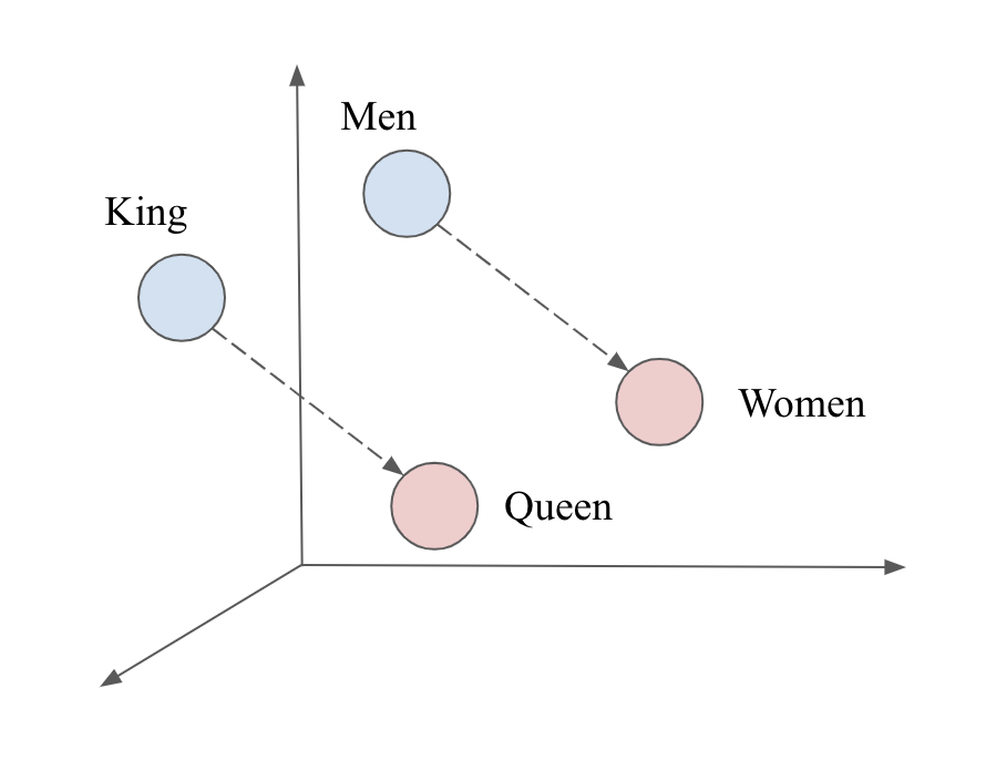
Since Word2Vec measures the similarity between words using Cosine similarity, we can see from the above vector space that the word King is similar to Queen, and Men is similar to Women.

Doc2Vec

Similar to Word2Vec, Doc2Vec turns a whole document/paragraph into numerical representations instead of word representations. If we can obtain one corpus from each of the apps by applying metapath2vec, then we can treat each corpus as its own document, and then feed it into the Doc2Vec model to learn representations for each of the documents. These vector representations can then be used in the classification process.

Data

The data we will be using is randomly downloaded from APK Pure and AMD malware dataset. It consists of labeled malware and other popular and unpopular (random) applications. Among our random apps downloaded from APK Pure, there might be one app out of five that might be a malware since they are apps that have little or no reviews. Rather than using .SMALI files, we will be working with APK files directly. From the APK files, we will be extracting a new form of representation called Control Flow Graphs. With APK files, we can easily generate control flow graphs through Androguard, which is a powerful tool to disassemble and decompile Android applications.

Control Flow Graphs

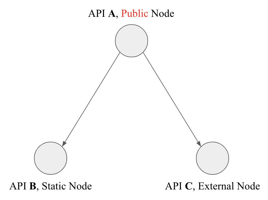
A Control Flow Graph (CFG) is a representation using graph notation of all paths that might be traversed through a program during execution. Firstly, a CFG consists of nodes and edges. Control Flow is the order in which individual statements, instructions, or function calls of an imperative program are executed or evaluated. Imperative meaning statements that change a program’s state. Each node in the CFG represents a basic block, or a straight-line piece of code without any jumps or jump targets. In our case, a node in the CFG is an API or method call. A jump statement is a statement that changes the program’s flow into another place of the source code. For example, from line 4 to line 60, or from file 1 to file 6. The following figures are two simple control flow graphs.

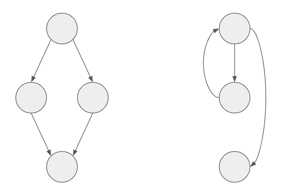
A node in our CFG can call another API (node). A node can be visualized as one of the circles in Figure 4, and the “call” action can be visualized by the arrow(edge). Each node has attributes. There are 7 Boolean attributes for each node, and 3 different edge types.

Node Attributes
External	If a node is an external method
Entrypoint	If a node is not called by anything
Native	If a node is native
Public	If the node is a public method
Static	If the node is a static method
Node	If none of the above are True
APK Node	If the node is an APK

We can pick from the 6 Boolean attributes and create node types based, such as: “external, public Node”, “external, static Node” and “entrypoint, native Node”. There can be more than 20 different node types.

Edge Types
Calls	API to API
Contains	APK to API
In	API to APK

Together, nodes and edges can build paths like: “external, public Node - calls -> external, static Node” or “APK - contains -> external, public Node”. The following is a control flow graph example with code block to explain how nodes are called:

Class: Lclass0/package0/exampleclass; ## let’s call this A
# direct methods
.method public constructor <init>()V
    if ....:
    	# api, call this B:
    	Lclass1/package1/example;->doSomething(Ljava/lang/String;)V
	else:
    	# api, call this C:
    	Lclass2/package2/example;->perform(L1/2/3)F

The method constructor calls API A, which calls API B: doSomething and calls API C: perform. Since API B and API C will jump to other places within the source code, the flow of the program is broken, and this jump is recorded in the control flow graph.

The Control Flow Graph from an app records tens of thousands of these calls, and represents them as edges, where each edge contains two nodes.

Common Graph

Since we obtained a large number of CFGs for a large number of APKs, we need to figure out a way to connect all of these graphs so the representations for each API will be the same. We want the API representations to be the same so when we are classifying we know that all feature vectors are built the same way. This is to avoid us creating random feature vectors, and will result in the model classifying randomly. To make sure we are building features correctly, we must create a common graph that links every CFG together. Also, during the testing phase, we can use these node embeddings to build a feature vector for an unseen app.

The common graph we built contains a total of 1,950,729 nodes, and 215,604,110 edges. Our common graph is simply a union of all the control flow graphs that we obtained from separate apps. This is not only to make sure that each distinct API node are consistent throughout our training and testing process, but to make sure that all our CFGs are on the same space. First, all the edges of each separate graphs are extracted, along with their weights and node types of each edge. Then, these information are loaded altogether to become a common graph.

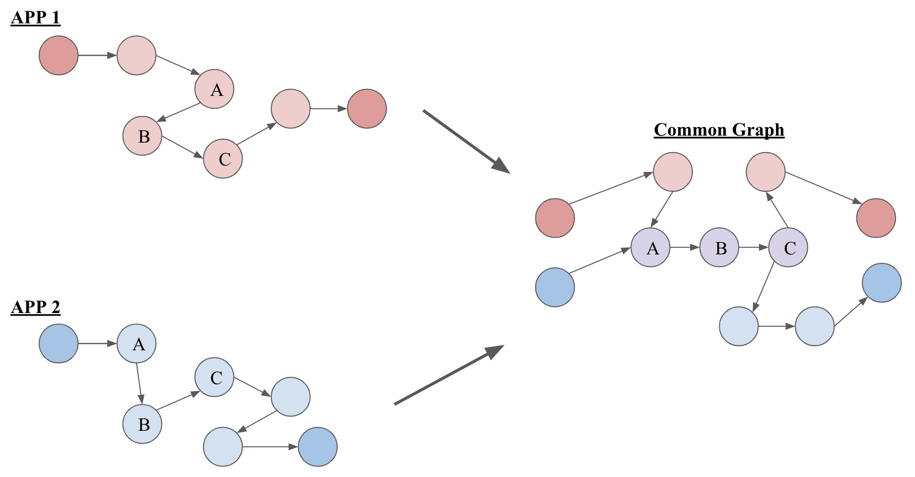
The figure above demonstrates what a common graph looks like by combining two control flow graphs from two different apps. On the left we have red and blue applications, which both have five nodes consisting of A, B, and C nodes connected together and other nodes of its own. When combining them, we generate the graph on the right, which merge the shared nodes with each other. Duplicate nodes are joined to be one, while the edges are still preserved. As you can see, the similar A, B, C sequence is preserved as well. This is important when we are building feature vectors for an app. The common graph ensures the same node representations for two graphs. This means that when we are building feature vectors for apps, the same representations are used for two similar apps. Conversely, if two apps are not similar and do not share the same sequences, then their representations will be very different. Like in the common graph in Figure 6, this will make sure that the similarity and differences between the apps are preserved.

Data Generating Process/ETL

The raw data we are investigating is code written by app developers. In order to turn something into a malware, you have to alter the source code, which will allow hackers to plant certain types of malicious code. If a developer were to hijack a device, then the app would need special Root permissions. Often targeting API calls that represent System Calls is one of the ways to alter the source code. For that reason, source code is an essential part in determining whether an application is malicious or not.

As mentioned above, we will be using control flow graphs converted directly from the APK files. We are looking at the sequence of which these system calls are made and define them as meta paths. We were able to obtain one CFG for each APK. We extracted this by using Androguard’s AnalysisAPK method in its misc module which returns an analysis object. Afterwards, we called .get_call_graph() on the analysis object to obtain the CFG. At this stage, we also perform some feature extraction specifically on the nodes of the graph. We extract the string representation of these nodes as well as node type. The string representations of nodes is used to build the corpus, and the node type is used to build meta paths. We then exported this graph as a compressed gml file to save on disk. We hypothesize that our method will perform better than our baseline model, since metapath2vec can capture the relations and context within the graphs, giving the feature vector much more information. Also, our metapaths are traversed in the beginning of our process to learn all possible metapaths. Using this method, we ensure that the model learns the different sequences that a malware could have, and use this information in future classification.

EDA

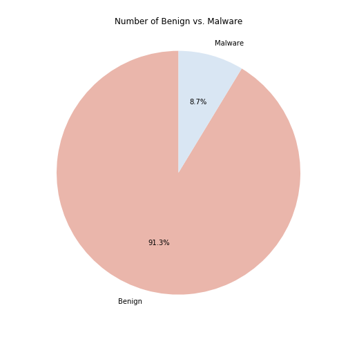
We have a total of 8435 malicious software and a total of 802 benign applications, which is a combination of popular apks and random apps. While generating control flow graph objects from the APK files, there was an error of “Missing AndroidManifest.xml,” so we were not able to generate those graphs and will be working with fewer benign apps \footnote{We looked into why there might be missing Android Manifest files error, interestingly, we found that some of the apps having this issue contain the manifest while some do not. However, the apps that have this issue do not decompile correctly, and do not create a graph correctly as well.}. To counteract the imbalance between malware and benign apps, we calculated class weights and used it in the classification process to ensure we are penalizing the model in a balanced way.

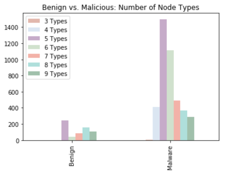
To further understand our benign and malicious data, we perform analysis on these graph objects by comparing the node types, as well as the counts of both nodes and edges.

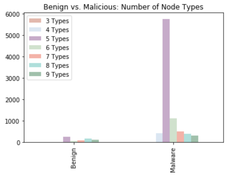
The figure above shows the comparisons of node types between benign applications and malicious code. From the two distributions, we can see that malware contains a lot more types of nodes compared to benign apps. Specifically, most of the malware contains five types of node. If we limit the range of that bar, we can see the figure below for a more clear distribution of benign apps. The left distribution also indicates that majority of the benign apps have five types of nodes.

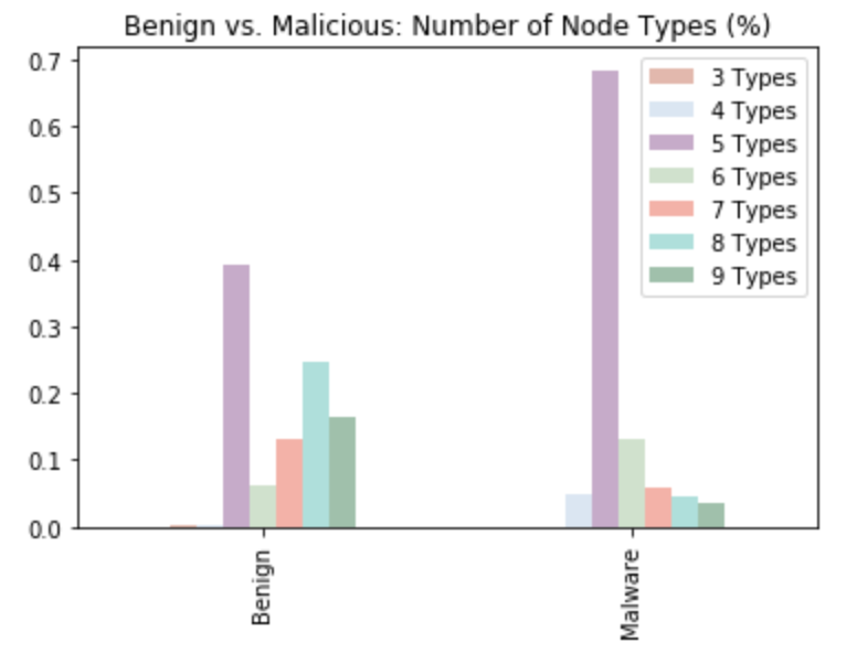
But because of how imbalanced our data is, we plot the number of node types based on the percentage, as shown in the below figure. From this figure we can conclude that over half of both benign and malicious apps have more than 5 types of nodes.

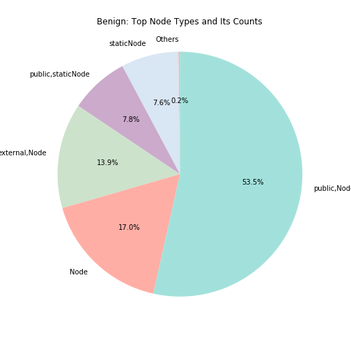
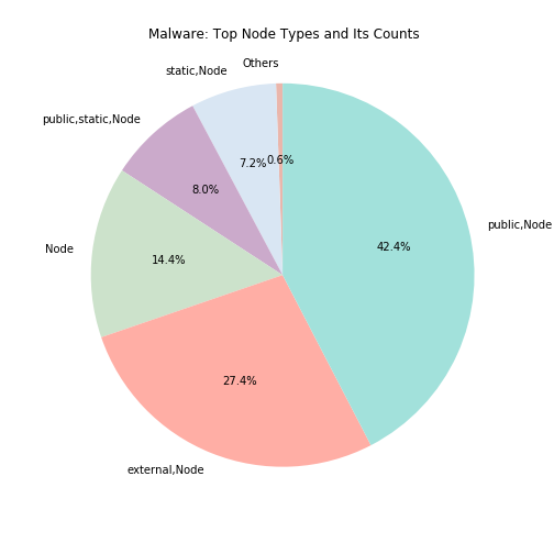
To further look into what are these node types, we analyze the top node types from both benign and malware separately. The following figures are node types distributions. On the left shows the benign node types spread, which over 50\% of the nodes are Public Node, followed by Node, External Node, Public Static Node, Static Node, and the other types. Similarly, for malware, Public Node is the top most node type found in the graphs. Followed by External Node, Node, Public Static Node, Static Node, and the others. Both benign and malware have similar top nodes.

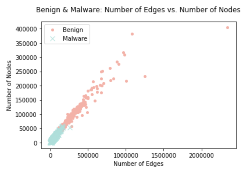
The figure below is a scatter plot of number of edges and number of nodes for both benign (red) and malware (blue). Although it seems that benign has a lot more apps in this plot, malware are just all packed together. We can also see that benign apps have larger number of edges and nodes compared to malware, this is because benign apps are larger in terms of APK sizes and that they might be more complicated.

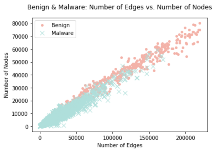
Since the figure above has outliers for benign apps and we want to focus on the malware, we limit the range so that it looks like the figure below. From this figure we see that malware is indeed packed together and that they have a lot less edge and nodes compared to the benign apps.

Methods

Feature Extraction

For our baseline, we extract probabilistic sequences from all possible edges of the APK, which serves as the feature vector for classification. For the Metapath2Vec model, we first create a common graph, then traverse it using Metapath2Vec to learn representations of nodes, which is used to build feature vectors. For our Doc2Vec method, we treat each APK as one document, and Doc2Vec produces one feature vector for one document.

Baseline: Mamadroid

We build Mamadroid as our baseline model. As introduced earlier, it extract call graphs that are represented using nodes and edges. With the graphs, it extracts all the possible edges based on the family or package level. It then extract sequences of probabilities of the edges occurring. This probabilistic feature vector is used for classification. We abstract API calls to both Family and Package level.

For example,

Example API call = "LFamily/Package"
Family Level = "LFamily"
Package Level = "LFamily/Package"

In Family level, there are seven possible families and 100 total possible edges. However, in Package level, there are 226 possible packages and a total of 51,239 possible edges. The number of possible families and packages are found on Android’s Developers page. Those families and packages that are not found on that webpage is abstracted to “self-defined”. Specifically, in family level, we will obtain a feature vector of 100 elements for one app. In package level, we obtain a feature vector with 51,239 elements for one app. These feature vectors are then used for classification. After obtaining the vector embeddings, we classify using Random Forest model, 1-Nearest Neighbors, and 3-Nearest Neighbors.

Metapath2Vec Model Using Common Graph

As mentioned earlier, we also abstracted our API calls to the class level. For example, an API call looks like this: “Lfamily/package/class; → doSomething()V” at the class level, it is: “Lfamily/package/class;”. The reason for this is there could be user-defined classes, which is not picked up in MamaDroid. We hope that we can obtain more information by abstracting to the class level, but not get too much information at the API level which might result in performance issues. We do not abstract anything to be “self-defined” as MamaDroid has.

1. Run a Depth First Search to explore all the node types that could be in an APK, and create metapaths.
2. Build a common graph by combining all the separate control flow graphs representing different apps.
3. Perform an uniform metapath walk on the common graph to obtain a huge corpus.
4. Perform node2vec to learn node representations of the huge corpus.
5. Build feature vectors for each app, using the node embeddings learned from step 3, by combining embeddings of unique nodes of each app.
6. Classification using built feature vectors.

Explanations: We run a depth first search to explore all node types and metapaths since we do not know how convoluted an app’s CFG may be and we need flexible metapaths for each app. Also, there is the possibility of the malware being intentionally obfuscated. Therefore, we need flexible metapaths for each app, which we will later use as the predefined metapaths in our metapath2vec step. The reason our feature vector is a component wise combination of node embeddings is because when two vectors are added together, a new vector is obtained. As visualized below:

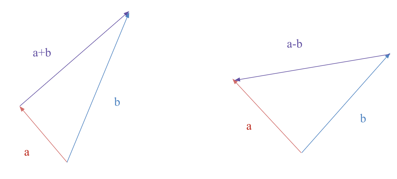
This will provide more information about the APKs that we will classify. The model can more easily learn the distinction between similar and different vectors, by the direction and magnitude to where they point. Of course, the component wise combination can also be other aggregations, such as taking an average, percentiles, and dot products. When encountering an unseen app, unique nodes of that app is extracted. Representations of each of the unique nodes are then found from the trained word2vec model, and some component wise combination is performed to obtain a feature vector for classification.

Doc2Vec Model

1. For each app, extract all possible metapaths using Depth First Search, as well as perform metapath2vec on that app to obtain a corpus.
2. Take each corpus from each app, append them, and turn them into a list of Tagged Documents.
3. Run the Tagged Documents into Doc2Vec to obtain a vector representation for each app.
4. Take the vector representations for each tagged document, and use them as feature vectors for classification.

The Doc2Vec model is very straight forward, taking in documents and returning representations for those documents. When there is an unseen app, a corpus is extracted from that app using metapath and is treated as a document. This document is then fed into the Doc2Vec model, and a vector representation is “inferred” using the .infer_vector() method.

Results and Analysis

Baseline Results

The following tables are results from our baseline model, MamaDroid, corresponding to Family and Package mode. Surprisingly, our MamaDroid using control flow graphs performs better than its original model. Let’s first take a look at the Family mode. The table below is the confusion matrix, we calculated precision and recall scores based on it.

	Random Forest	1-NN	3-NN
True Negative	68	61	59
False Negative	4	9	8
False Positive	11	18	20
True Positive	1269	1264	1265

We compare the results to the original MamaDroid model. In the table below, we list the original MamaDroid results on it as well to better compare it. We see that our version of MamaDroid has better performance in all F1-Score, precision and recall scores, where we obtain an F measure of 0.994 and the original model only has 0.880. Similarly to precision and recall scores, we obtain 0.991 and 0.997, where the original model has 0.840 and 0.920 as their results. In addition to Random Forest, our 1-NN and 3-NN models also outperform the original MamaDroid model. But all our three models have similar results.

PCA = 10 Component	Random Forest		1-NN	3-NN
	Original	Ours
F1-Score	0.880	0.994	0.980	0.994
Precision	0.840	0.991	0.985	0.994
Recall	0.920	0.997	0.994	0.994

Next, we have results for our MamaDroid Package mode. The following table is the confusion matrix. The numbers are close to what we obtain for Family level. However, the true negatives for all three similarity-based models are slightly larger.

	Random Forest	1-NN	3-NN
True Negative	70	70	70
False Negative	1	6	1
False Positive	15	15	15
True Positive	1266	1261	1266

We also compared the results of Package mode to the original MamaDroid results. In the table shown below, we also list out the results of original MamaDroid on the left to compare it with the ones we obtain. As a result, our model was able to achieve an F measure of 0.993, precision score of 0.988, and recall score of 0.999, whereas the original model only has performance of 0.940, 0.940, and 0.950. Both 1-NN and 3-NN models also have very similar numbers as Random Forest model.

PCA = 10 Component	Random Forest		1-NN	3-NN
	Original	Ours
F1-Score	0.940	0.993	0.992	0.994
Precision	0.940	0.988	0.988	0.988
Recall	0.950	0.999	0.995	0.999

Metapath2Vec/Common Graph (Partial)

For our Metapath2Vec model, we unfortunately do not have the complete results due to large computational time it takes to build the common graph with all the data we have. The complete common graph consists of 1,950,729 nodes, and 215,604,110 edges. However, we did obtain results working with a smaller subset of the Common Graph, consisting of: 87,539 nodes and 15,617,223 edges.

	Random Forest	1-NN	3-NN
True Negative	94	89	73
False Negative	16	31	36
False Positive	20	25	41
True Positive	1679	1664	1659

We tested on the entire test set, and surprisingly the performance was okay. Initially, we thought that there might be an error, however, upon inspecting our code, we were traversing the smaller common graph correctly. We believe we can obtain this result because of the large amount of edges in the common graph as well as our walk length of 500. We set the walk length to 500 to compensate for the smaller subset of graphs that we are using, and therefore can capture more information per walk. Because of this, the Word2Vec model can learn more about those nodes and provide a better representation.

	Random Forest	1-NN	3-NN
TF1-Score	0.989	0.983	0.977
Precision	0.992	0.966	0.982
Recall	0.642	0.959	0.959

Even though the F1-Scores were high, our True Negative and False Positives are higher than our baseline and Doc2vec model. This is again due to the smaller subset that we are using for this experiment. Because of the smaller subset, we do not have a lot of representations for nodes. There could have been some nodes that the word2vec model has never seen before, and therefore cannot infer a good representation for it.

Doc2Vec

The following tables are the results for Doc2Vec with our similarity-based models: Random Forest, 1-NN, and 3-NN. Table below is the confusion matrix, which is used to compute the precision and recall scores. The Doc2Vec performed worse than the baseline model on the Random Forest model, and it seems like it was struggling with classifying benign apps.

	Random Forest	1-NN	3-NN
True Negative	109	56	43
False Negative	606	68	71
False Positive	5	58	31
True Positive	1089	1627	1664

In the table below, we have our F measure, precision, and recall scores. We notice that our Random Forest model only has an F measure of 0.781, which is a lot lower than our baseline. On the other hand, both our k Nearest Neighbors perform much better than Random Forest. The Random Forest classifier has an emphasis on certain features when training, and focuses on some feature more than others. However, the 1-NN and 3-NN models both look at an unseen vector’s closest neighbors, therefore utilizing all the features in the vector. We believe this is why the 1-NN and 3-NN models performed better in this experiment.

	Random Forest	1-NN	3-NN
TF1-Score	0.781	0.963	0.970
Precision	0.992	0.966	0.982
Recall	0.642	0.959	0.959

Conclusion

In conclusion, our baseline model is able to achieve a better performance than the original work that we have studied. Although our Doc2Vec did not perform better than the baseline Random Forest model, our k Nearest Neighbors models performed almost as good as our baseline. From this, we can see that Control Flow Graphs might be a good choice when it comes to choosing representations for source code. Again, control flow graphs show the jumps in code. From our EDA: Figure 12, even though malware has a small number of nodes, they have a large amount of edges. This means that there could be lots of instances where the program is jumping around in the source code. All this is recorded in the CFG representation and could provide much more information about an APK.

Although we successfully created a complete common graph, we were unable to obtain all the node embeddings from it due to time and memory constraints. Therefore we built a smaller common graph to see how it performs. If time and resources allowed, we hope to finish the metapath traversal of the complete common graph. Judging from the results using the smaller common graph, if we were to scale up the model might out-perform our baseline.

For our future work, we plan on investigating other vector embeddings technique and perhaps instead of using only similarity-based models, we could also implement graph neural networks (GNN). In addition to neural networks, we are also interested in graph classification specifically. Since our data format is already in the form of multiple apps, it can be easy to normalize and transform data for a GNN model. Of so many researches we have seen on malware detection, not a lot of them uses control flow graphs as their input data. Since our experiments confirmed that using control flow graphs is not any worse than using other forms of data, we are curious to know if control flow graphs can outperform in other models.

Acknowledgement

We would like to express our gratitude to our mentors for our Capstone project: Professor Aaron Fraenkel, who provided us with lots of resources and ideas throughout the entire process of our research, and Shivam Lakhotia, who guided us through the project and assisted us every week.

References

[1] MamaDroid, https://arxiv.org/pdf/1612.04433.pdf

[2] Hindroid, https://www.cse.ust.hk/~yqsong/papers/2017-KDD-HINDROID.pdf

[3] Metapath2Vec, https://ericdongyx.github.io/papers/KDD17-dong-chawla-swami-metapath2vec.pdf

[4] Word2Vec, https://radimrehurek.com/gensim/models/word2vec.html

[5] Doc2Vec, https://radimrehurek.com/gensim/models/doc2vec.html

[6] Androguard, https://androguard.blogspot.com/2011/02/android-apps-visualization.html

[7] StellarGraph, https://github.com/stellargraph/stellargraph

[8] SDK, https://developer.android.com/studio/releases/platforms

[9] x2vec, https://iopscience.iop.org/article/10.1088/2632-072X/aba83d/pdf

[10] Learning Embeddings of Directed Networks with Text-Associated Nodes—with Application in Software Package Dependency Networks, https://arxiv.org/pdf/1809.02270.pdf